When working with large Excel spreadsheets, it’s easy to lose track of your column headers as you scroll down. Freezing the top two rows in Excel helps keep your key information in view, improving clarity and saving you time. Whether you’re dealing with financial reports, project trackers, or massive datasets, this small trick can make a big difference.
What Is the “Freeze Panes” Feature?
“Freeze Panes” is an Excel feature that locks specific rows or columns in place, allowing you to scroll through the rest of your data while keeping the frozen areas visible. Once activated, a gray line appears below the frozen rows, signaling the locked position.
It’s important to distinguish between Excel’s “Freeze Top Row” option, which locks only the first row, and the more flexible “Freeze Panes” option, which allows you to freeze multiple rows or columns based on your selection. This is particularly useful when you want to freeze the top two rows in Excel to keep both headers and subheaders visible.
Step-by-Step: Freeze the Top Two Rows in Excel
Manual Steps
- Open your Excel spreadsheet.
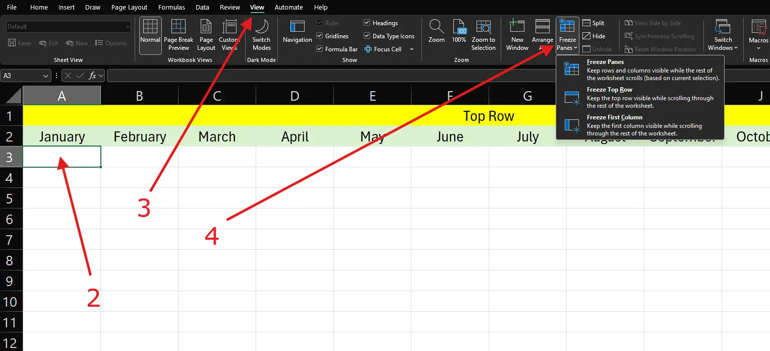
- Click to select cell A3.
- Go to the View tab on the Ribbon.
- Click Freeze Panes, then select Freeze Panes from the dropdown menu.
That’s it! Rows 1 and 2 are now locked in place.
Keyboard Shortcut Tip
On Windows, quickly freeze panes by selecting cell A3 and pressing Alt + W + F + F. This shortcut speeds up the process compared to manually navigating the Ribbon.
How Can You Confirm the top 2 Rows Are Frozen?
After freezing the rows, you’ll notice a gray horizontal line appear beneath Row 2. This line indicates where the scrolling split begins, everything above it is now frozen. If you’ve properly followed the steps to freeze the top two rows in Excel, this visual cue confirms the success.
Top 2 rows not frozen
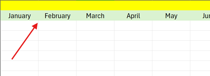
Top 2 rows frozen (darker horizontal line between rows 2 and 3)
What Are Some Additional Use Cases?
Freezing Both Rows and Columns
You can freeze both rows and columns at the same time. To do this:
- Click the cell below the last row you want to freeze and to the right of the last column you want to freeze. For example, to freeze Rows 1 and 2 and Columns A and B, select cell C3.
- Go to View > Freeze Panes > Freeze Panes.
This locks the specified area and allows you to scroll through the rest of your sheet freely.
Why Is “Freeze Panes” Not Working and How Can You Fix It??
- “Freeze Panes” is greyed out? Make sure you’re in Normal View (check under the View tab) and not editing a cell.
- Hidden or filtered rows? Ensure the rows you want to freeze are visible before applying the Freeze Panes setting.
- You’re selecting the wrong cell? Always select the cell just beneath and to the right of what you want to freeze.
Extra Tips and Tricks
Best Practices Suggestion
After freezing rows, it’s a good idea to apply filters or use bold or colored formatting on your header rows. This not only improves visual clarity but also ensures consistency, especially when the sheet is shared with others.
Bonus Tip: How to Unfreeze Top Two Rows in Excel
If you need to undo freezing at any point, it’s simple:
- Go to the View tab.
- Click the Freeze Panes dropdown.
- Select Unfreeze Panes.
You can also quickly unfreeze panes by pressing Alt + W + F + F anywhere on the sheet.
Why Should You Freeze the Top Two Rows in Excel?
Freezing the top two rows in Excel is a simple but powerful technique to keep your headers visible as you scroll. It enhances navigation, boosts productivity, and helps prevent errors. Pair this feature with filters or Excel Tables for an even more efficient workflow.
Now that you know how to use Freeze Panes like a pro, try freezing the top two rows in Excel in your next spreadsheet and experience the difference!