XLOOKUP is a powerful lookup function available in both Excel and Google Sheets. It offers a flexible, intuitive way to search and return data without many of the limitations found in older lookup methods. Whether you’re working with small tables or large datasets, XLOOKUP helps you locate information cleanly and reliably.
It also works across devices and platforms, making it a consistent and dependable choice for users in both Excel and Google Sheets.
In both Excel and Google Sheets, XLOOKUP improves accuracy, prevents formula failures after structural changes, and provides more control over how matches are found. These improvements make it the modern standard for anyone working with data lookup tasks.
What Is the XLOOKUP Syntax?
XLOOKUP uses six total arguments—three required and three optional. Both Excel and Google Sheets use the same syntax, making it easy to work across tools.
=XLOOKUP(lookup_value, lookup_array, return_array, [if_not_found], [match_mode], [search_mode])Required Arguments
- lookup_value: The value you want to find in your dataset.
- lookup_array: The range where the function searches for the lookup value.
- return_array: The corresponding values to pull from once a match is found.
Optional Arguments
- if_not_found: Custom text or value to return instead of an error. You can leave this blank by inserting an extra comma:
,,. - match_mode: Controls exact, approximate, wildcard, or regex matching. If you want to skip this and use the next argument, keep the comma placeholder:
,,0. - search_mode: Allows normal, reverse, or binary searching. To use search_mode without using match_mode, add a comma to hold its position.
How to Use Optional Arguments Selectively
XLOOKUP lets you skip optional arguments by keeping the commas that mark their positions. This means you can jump directly to later options like match_mode or search_mode without filling the earlier ones.
Examples:
- Use search_mode but NOT if_not_found or match_mode:
=XLOOKUP(A1, B2:B10, C2:C10,, , -1) - Use match_mode but skip if_not_found:
=XLOOKUP(A1, B2:B10, C2:C10,, 0) - Use both match_mode and search_mode:
=XLOOKUP(A1, B2:B10, C2:C10,, 0, -1)
This makes XLOOKUP extremely flexible, letting you control only the arguments you care about while leaving others at their default settings.
Together, these arguments give you much more control than older lookup functions ever offered.
How Is XLOOKUP Better Than VLOOKUP?
Left Lookup Capability
One of the biggest advantages is the ability to search in any direction. VLOOKUP can only search rightward from the lookup column. But XLOOKUP can look left, right, up, or down in both Excel and Google Sheets.
Exact Match by Default
VLOOKUP defaults to approximate matching, which frequently leads to incorrect results if you forget to adjust the formula. XLOOKUP defaults to exact matching, the correct choice for most real-world scenarios.
Column Stability
Instead of relying on a fragile column index number, XLOOKUP directly references the return range. This means your formula won’t break if you insert, delete, or rearrange columns—an advantage for anyone maintaining evolving spreadsheets.
Integrated Error Handling
With the if_not_found argument, you no longer need to wrap your lookup in IFERROR. Just define your custom message directly inside XLOOKUP.
Vertical and Horizontal Lookups
XLOOKUP replaces both VLOOKUP and HLOOKUP. You only need one function for any lookup direction.
Improved Performance
Since XLOOKUP only calculates the necessary arrays instead of entire table ranges, it can be significantly faster than VLOOKUP, especially in medium-to-large datasets. This performance benefit applies to both Excel and Google Sheets.
How Do You Use XLOOKUP? (Basic Examples)
Exact Match Example
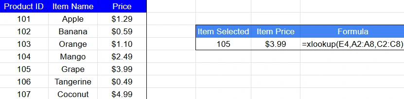
=XLOOKUP(E4, A2:A8, C2:C8)This formula checks the value in E4, scans the range A2:A8 for a match, and returns the value in C2:C8 that aligns with it. It’s a clean, easy-to-read lookup suitable for product lists, employee directories, or category tables.
Missing Values Example
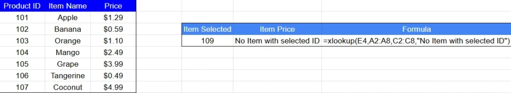
=xlookup(E4,A2:A8,C2:C8,"No Item with selected ID")Instead of an error message like #N/A, you can return friendly text such as “No Item with selected ID” improving readability and user experience.
Returning Multiple Columns
XLOOKUP supports spill behavior in both Excel and Google Sheets. If your return array covers multiple columns, the results spill across adjacent cells.
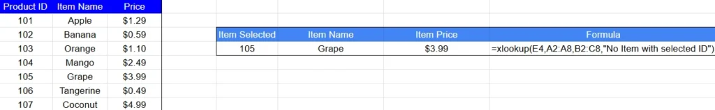
=xlookup(E4,A2:A8,B2:C8,"No Item with selected ID")This will output two columns of data at once. In this case, XLOOKUP returns both item name and item price.
What Are XLOOKUP Match Modes?
Approximate Match (-1 and 1)
Approximate matches are great when working with tiers or scoring boundaries.
- -1: Finds exact match or next smaller value.
- 1: Finds exact match or next larger value.
These are essential for tasks like pricing tables, commission structures, and grading systems.
Wildcard Match (2)
Wildcards help you search partially matched text:
=XLOOKUP("*"&E1&"*", A2:A8, B2:B8, , 2)The * symbol represents any number of characters, letting you find results based on partial names, product codes, or descriptions.
Regex Match (3)
Excel 365 offers regex-based matching through XLOOKUP, allowing advanced pattern identification. Google Sheets supports regex too, though typically through functions like REGEXMATCH; however, XLOOKUP in Sheets also supports regex mode.
This is useful for validating formats, decoding structured text, or filtering complex datasets.
How Do You Control XLOOKUP Search Direction?
Standard Search (1)
Forward search — the default mode — moves top to bottom or left to right.
Reverse Search (-1)
To find the last occurrence instead of the first, use reverse search:
=XLOOKUP(A2, B2:B20, C2:C20, , 0, -1)Binary Search (2 or -2)
Binary search is incredibly fast but requires sorted data. It’s ideal when working with massive datasets, especially in Excel.
How Can You Use XLOOKUP for Advanced Tasks?
Multiple Criteria Lookups
By combining conditions with Boolean logic, you can perform multi-criteria lookups:
=XLOOKUP(1, (A2:A20=H1)*(B2:B20=H2), C2:C20)   # Excel

=XLOOKUP(1, ARRAYFORMULA((A2:A20=H1)*(B2:B20=H2)), C2:C20)   # Google Sheets
This checks for rows where both conditions are true.
For Google Sheets, XLOOKUP does not natively evaluate array logic the way Excel does, so the second argument must be wrapped in ARRAYFORMULA for the function to process multiple rows correctly.
Two-Way (Nested) XLOOKUP
You can use a nested XLOOKUP to find results at the intersection of a row and column:
=XLOOKUP(A2, A5:A20, XLOOKUP(B1, B4:F4, B5:F20))This technique is ideal for matrix-style data like budgets, schedules, or pricing grids.
Case-Sensitive Lookups
To make XLOOKUP case-sensitive, wrap the lookup array with the EXACT function:
=XLOOKUP(TRUE, EXACT(A2:A20, H1), B2:B20)   # Excel

=XLOOKUP(TRUE, ARRAYFORMULA(EXACT(A2:A20, H1)), B2:B20)   # Google Sheets
This allows you to distinguish between values like “codeA” and “codea”—something normal XLOOKUP won’t do by default.
For Google Sheets, you must wrap the EXACT function inside ARRAYFORMULA or XLOOKUP will only evaluate the first row.
How Do You Fix Common XLOOKUP Errors?
#N/A Error
This error appears when the lookup value doesn’t exist in the lookup array. Double-check your value or add an if_not_found argument.
#VALUE! Error
This occurs when your lookup and return arrays don’t have matching dimensions. Make sure the ranges line up correctly.
#REF! Error
If you’re referencing an external workbook that’s closed, Excel can’t pull the values and returns a #REF! error. This error can also occur if cells were deleted, shifted, or the referenced range no longer exists.
Incorrect Results
Often caused by formulas that weren’t adjusted with absolute references ($). Lock your ranges when copying formulas.
Performance Issues
Extra-large datasets may calculate more slowly. You can optimize performance by using smaller lookup ranges or turning off unnecessary calculations.
Why Use XLOOKUP Going Forward?
XLOOKUP is the modern replacement for older lookup functions in both Excel and Google Sheets. It’s more accurate, easier to maintain, and more powerful. Whether you’re working with product lists, financial models, inventory systems, or reports, XLOOKUP gives you the flexibility and control needed to keep your spreadsheets clean, reliable, and efficient.
To deepen your skills even further, explore related functions like FILTER, XMATCH, INDEX MATCH, and UNIQUE—each pairs beautifully with XLOOKUP for advanced data analysis and cleaner spreadsheet design.