If you’ve ever wanted cells in Google Sheets to automatically change color based on values somewhere else in your spreadsheet, you’re in the right place. Google Sheets conditional formatting based on another cell is one of the most powerful (and misunderstood) features in spreadsheets. Once you understand how it works, you can build dashboards, trackers, schedules, and reports that visually update themselves in real time.
This guide explains the concept clearly, shows when and why to use it, and walks through practical patterns you’ll actually reuse. It’s written for beginners who want confidence and intermediate users who want fewer surprises.
When should you use conditional formatting based on another cell?
This approach is ideal when one column controls behavior for other columns. Common real-world scenarios include project trackers where a Status column determines row color, financial sheets where totals are compared against a fixed budget cell, attendance or habit trackers where checkboxes affect labels or dates, and schedules where one date column flags another.
If your formatting logic depends on relationships between cells rather than a single value, conditional formatting based on another cell is almost always the right tool.
How does Google Sheets evaluate conditional formatting formulas?
This is where many users get stuck. Conditional formatting formulas behave differently than normal spreadsheet formulas. Instead of calculating a visible result, they return TRUE or FALSE behind the scenes. If the formula evaluates to TRUE, the formatting applies. If it evaluates to FALSE, nothing happens.
Another important detail is relative referencing. Google Sheets evaluates the formula as if it starts in the top-left cell of the selected range, then adjusts references as it moves through the range. This means absolute references (using $ signs) matter a lot. One misplaced dollar sign can cause formatting to apply everywhere—or nowhere.
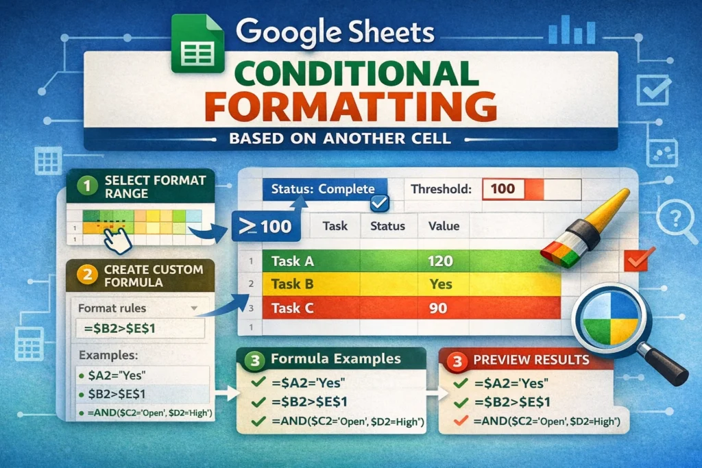
How do you set up conditional formatting based on another cell?
Start by selecting the range you want to format. This is the area that will visually change. Then open Format → Conditional formatting and choose “Custom formula is” as the rule type. Your formula should reference the controlling cell or column that determines the condition.
Always write the formula as if it applies to the first cell in your selected range. Google Sheets will handle the rest automatically if your references are set correctly.
Basic custom formula patterns you should know
Before diving into full examples, it helps to recognize a few core patterns. Comparisons like equals, greater than, and less than are the foundation. Logical functions like AND and OR let you combine multiple conditions. Functions like ISBLANK or LEN help handle empty cells gracefully.
Most conditional formatting formulas are short, simple, and focused. Complexity comes from understanding references, not from stacking many functions together.
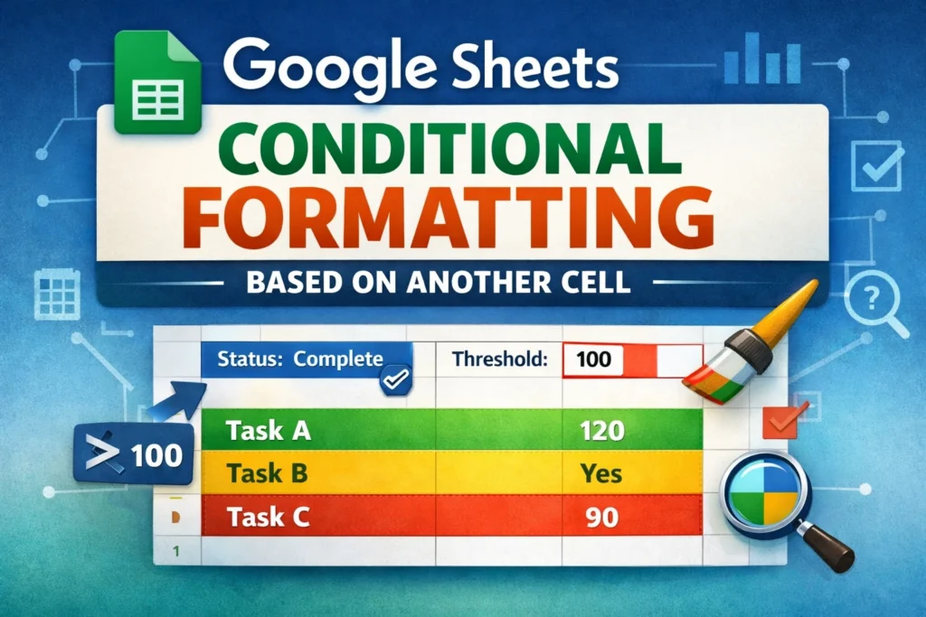
Conditional formatting based on another cell value
This is the most common use case. One cell determines whether another cell (or range) is highlighted.
Custom Formula Examples
If you want to highlight cells in column B when column A contains “Yes”:
=$A1="Yes"This formula checks column A for each row and applies formatting to the corresponding cell in column B.
If you want to format an entire row based on a status in column C:
=$C1="Complete"Select the entire row range (for example, A1:F100) before applying the rule.
If you want formatting to trigger when a numeric value exceeds a threshold stored in another cell:
=B1>$E$1Here, E1 is locked so every row compares against the same reference value.
How to highlight a row based on one cell
Row-based formatting is extremely useful for trackers and dashboards. The trick is selecting the full row range and anchoring the column reference.
Custom Formula Examples
To highlight an entire row when a checkbox in column D is checked:
=$D1=TRUECheckboxes return TRUE or FALSE, making them ideal triggers for formatting.
To highlight overdue tasks when a Due Date column is earlier than today:
=$B1<TODAY()
This assumes column B contains due dates. The formatting applies across the row, but the condition is controlled by a single column.
How to use conditional formatting with text in another cell
Text-based conditions are especially helpful for labels like “High,” “Medium,” or “Low,” or workflow states like “In Progress.”
Custom Formula Examples
To format cells when another column contains specific text:
=ISNUMBER(SEARCH("urgent",$C1))This allows partial matches and avoids errors when text varies slightly.
For exact matches, a simple equality check is often better:
=$C1="Delayed"Exact matches are faster and more predictable than search-based logic.
How to use AND and OR with multiple conditions
Sometimes one condition isn’t enough. You may want formatting to apply only when several criteria are met.
Custom Formula Examples
To highlight a row only if status is “Open” and priority is “High”:
=AND($C1="Open",$D1="High")To apply formatting if either condition is true:
=OR($C1="Overdue",$C1="Blocked")Combining conditions keeps your sheet visually clean without adding helper columns.
Common mistakes that cause conditional formatting to fail
One of the biggest mistakes is selecting the wrong range. The rule might be correct, but if the range doesn’t match the formula logic, formatting won’t behave as expected. Another frequent issue is missing dollar signs, which causes references to shift incorrectly as the rule applies across rows or columns.
Users also often forget that conditional formatting formulas must return TRUE or FALSE. If your formula produces a number or text result, it won’t work. Lastly, overlapping rules can override each other. Google Sheets applies rules in order, so rule priority matters when multiple formats target the same cells.
Are there limitations to conditional formatting based on another cell?
Yes, and it’s important to understand them. Conditional formatting can’t directly reference cells in another spreadsheet. It also recalculates frequently, so extremely complex rules across thousands of rows can impact performance. Additionally, formatting rules don’t “store” results—if the referenced cell changes, formatting updates instantly, which is usually a benefit but can surprise new users.
For advanced logic, helper columns are sometimes clearer and more maintainable than extremely long formulas hidden inside formatting rules.
When should you use helper columns instead?
Helper columns are useful when logic becomes hard to read or debug. Instead of embedding complex calculations in conditional formatting, you can calculate TRUE or FALSE in a helper column and base formatting on that result. This makes spreadsheets easier to audit and reduces future confusion, especially when sharing files with others.
How conditional formatting fits into reusable templates
At Sheetrix, many downloadable templates rely on conditional formatting based on another cell to guide users visually without instructions. Status-driven row highlights, progress indicators, and alerts all make spreadsheets feel smarter and easier to use. Once set up correctly, these rules require no maintenance and work automatically as data changes.
Final thoughts on mastering conditional formatting based on another cell
Google Sheets conditional formatting based on another cell is less about memorizing formulas and more about understanding how Sheets evaluates conditions across ranges. Once you grasp relative references, TRUE/FALSE logic, and rule scope, you can build spreadsheets that communicate insights instantly.
Whether you’re managing tasks, tracking finances, or designing templates for others, this technique turns raw data into visual signals that save time and reduce errors. With a few well-placed rules, your spreadsheet can tell you exactly what matters—without you having to search for it.