If you’ve ever tried to look up data in Google Sheets and felt limited by VLOOKUP, learning how to use Google Sheets INDEX MATCH can completely change how you work with spreadsheets. INDEX MATCH is more flexible, more reliable, and better suited for real-world data that changes over time. While it can look intimidating at first, the concept is simpler than it seems once you understand how the two functions work together.
In this guide, you’ll learn what INDEX MATCH is, why it’s often preferred over VLOOKUP, how it works step by step, and how to avoid common mistakes. By the end, you’ll be able to use it confidently in everyday spreadsheets, templates, and reports.
What is INDEX MATCH in Google Sheets and why do people use it?

Google Sheets INDEX MATCH is a lookup method that combines two functions: INDEX and MATCH. Together, they allow you to find a value in a table based on a matching row or column, without the structural limitations of older lookup functions.
INDEX returns a value from a specific position in a range. MATCH finds the position of a value within a range. When you nest MATCH inside INDEX, the MATCH function figures out the row or column number, and INDEX uses that number to return the correct value.
People prefer INDEX MATCH because it works even when columns move, supports left-to-right and right-to-left lookups, and scales better in larger spreadsheets. It’s especially useful in dashboards, trackers, and templates where data structures change over time.
How does INDEX MATCH work conceptually?
The easiest way to understand INDEX MATCH is to separate the two jobs it performs. MATCH answers the question, “Where is this value located?” INDEX answers the question, “What value is stored at that location?”
Imagine you have a list of product names in one column and prices in another. MATCH scans the product column to find the position of the product you’re searching for. INDEX then uses that position to pull the corresponding price from the price column.
This separation is what makes INDEX MATCH so flexible. You are no longer forced to look only to the right of a column, and your formulas won’t break if someone inserts or rearranges columns later.
Why is INDEX MATCH better than VLOOKUP in Google Sheets?
VLOOKUP is popular because it’s simple, but it comes with several limitations that cause problems in real spreadsheets. INDEX MATCH avoids most of these issues.
First, VLOOKUP can only search from left to right. INDEX MATCH can look up values in any direction. Second, VLOOKUP relies on a fixed column number, which breaks if columns are added or moved. INDEX MATCH uses dynamic positions, so it keeps working even when your sheet changes. Third, INDEX MATCH can be more efficient in large datasets, especially when used carefully.
For anyone building reusable templates, financial trackers, or multi-sheet dashboards, INDEX MATCH is usually the safer long-term choice.
How do you write a basic INDEX MATCH formula?
Before diving into advanced scenarios, it’s important to understand the basic structure. INDEX MATCH always follows the same pattern: INDEX(range_to_return, MATCH(lookup_value, lookup_range, match_type)).
INDEX MATCH formula example
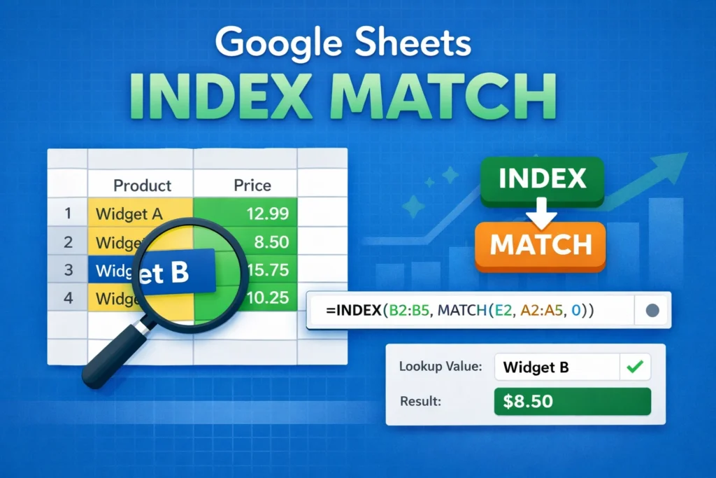
Here’s a simple example that looks up a value based on an exact match:
=INDEX(B2:B10, MATCH(E2, A2:A10, 0))
In this formula, B2:B10 is the column containing the value you want to return. E2 contains the lookup value. A2:A10 is the column being searched. The 0 tells MATCH to look for an exact match.
Once you understand this pattern, you can apply it to almost any lookup scenario in Google Sheets.
How can you use INDEX MATCH across different sheets?
One of the most common real-world uses of INDEX MATCH is pulling data from another sheet. This is especially useful in summary tabs, dashboards, or reports.
You simply reference the other sheet’s ranges inside the formula. As long as the ranges align properly, the logic stays exactly the same. This makes INDEX MATCH ideal for separating raw data from presentation sheets without duplicating information.
When working across sheets, always double-check that both ranges are the same size. Mismatched ranges are a frequent source of errors.
What are common mistakes people make with INDEX MATCH?
One of the biggest mistakes is mismatched ranges. The lookup range in MATCH must align with the return range in INDEX. If one range has extra rows or starts at a different row, the formula may return incorrect results or errors.
Another common issue is using the wrong match type. Leaving out the third argument in MATCH defaults to an approximate match, which can return unexpected results if the data isn’t sorted. For most use cases, you should explicitly use 0 for an exact match.
People also sometimes try to use INDEX MATCH where simpler functions would work better. While INDEX MATCH is powerful, it’s not always necessary for basic lookups in small, static tables.
When should you use INDEX MATCH instead of other lookup functions?
INDEX MATCH shines when your spreadsheet needs flexibility. If columns might move, if you need to look up values to the left, or if your sheet is part of a reusable template, INDEX MATCH is usually the best choice.
However, for very simple tasks, functions like VLOOKUP or XLOOKUP (where available) may be easier to read. The key is choosing the right tool for the job rather than defaulting to one function every time.
For conditional lookups involving multiple criteria, INDEX MATCH can be combined with other functions, but in some cases newer functions or helper columns may provide clearer solutions.