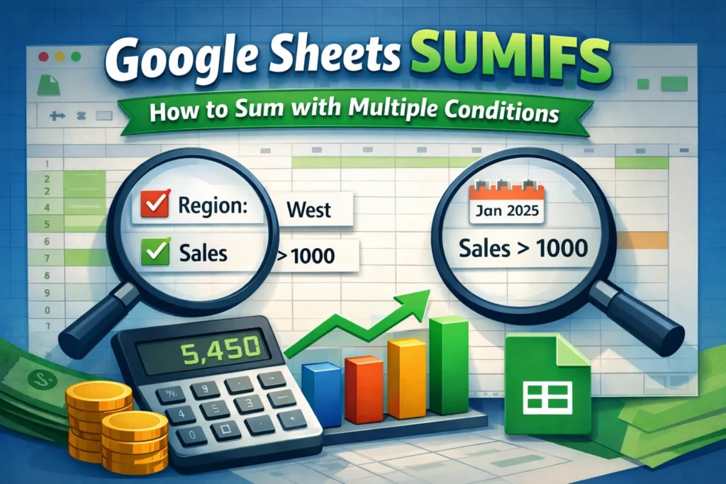
When you start working with real-world data in Google Sheets, you quickly realize that simple totals are rarely enough. You don’t just want to add numbers—you want to add specific numbers that meet certain rules. That’s exactly where Google Sheets SUMIFS shines. This function allows you to sum values only when multiple conditions are met, making it essential for budgets, sales reports, trackers, and dashboards.
This guide explains how SUMIFS works, when to use it, common mistakes to avoid, and how it compares to related functions, all in a clear, practical way.
What is the Google Sheets SUMIFS function and why is it useful?
SUMIFS is a conditional summing function. It adds numbers from a range only if all specified criteria are true. Unlike SUMIF, which supports just one condition, SUMIFS is designed for more complex scenarios where multiple filters matter at the same time.
For example, you might want to:
- Total sales from a specific region and a specific month
- Sum expenses for a single category and a specific payment method
- Add hours worked by one employee within a certain date range
SUMIFS helps you answer these questions without sorting, filtering, or manually calculating totals.
How does the SUMIFS syntax work in Google Sheets?
The structure of SUMIFS looks intimidating at first, but it follows a predictable pattern once you understand it.
SUMIFS syntax
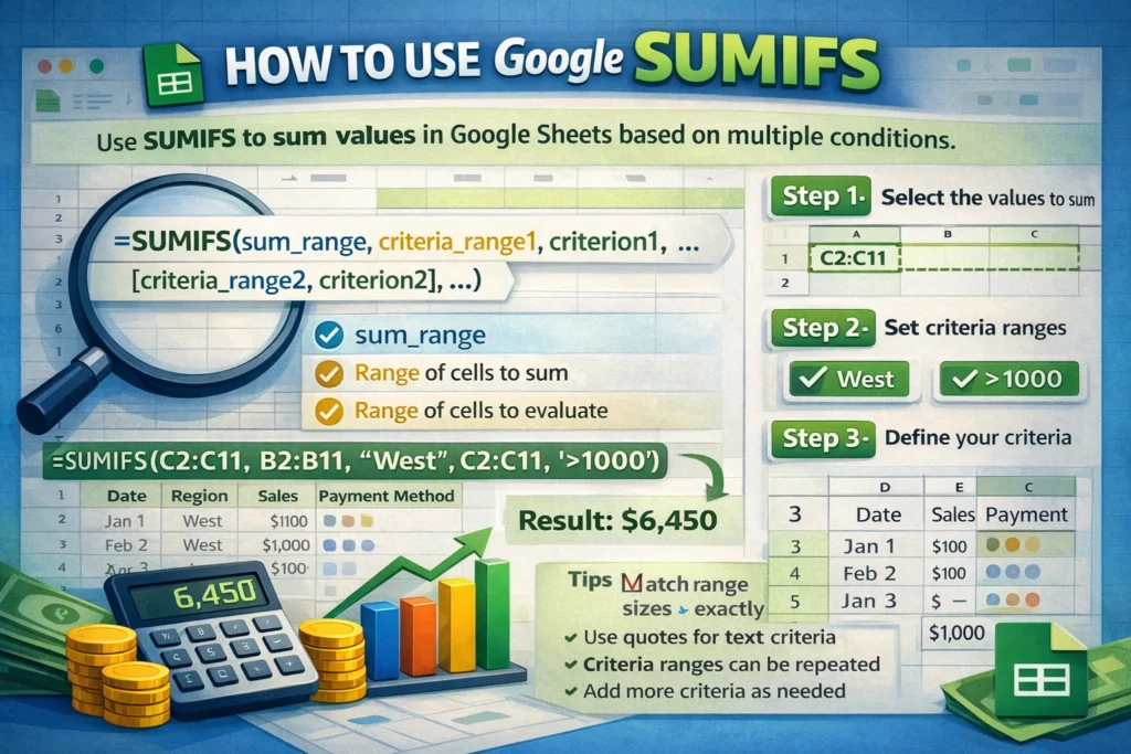
SUMIFS(sum_range, criteria_range1, criterion1, [criteria_range2, criterion2], ...)Here’s what each part means:
- sum_range: The cells containing the numbers you want to add
- criteria_range: The cells to evaluate against a condition
- criterion: The rule that must be met (text, number, date, or expression)
Every criteria range must be the same size as the sum range. Google Sheets evaluates each row and only includes values where all criteria are true.
When should you use SUMIFS instead of SUM or SUMIF?
Use SUMIFS when your total depends on more than one condition. If you only need a simple total, SUM is enough. If you need one condition, SUMIF works fine. But as soon as you add a second rule, SUMIFS becomes the right tool.
A common beginner mistake is trying to nest multiple SUMIF functions together. While this can sometimes work, it’s harder to read, easier to break, and less efficient than using one SUMIFS formula.
SUMIFS formula examples
Below are focused examples that show how SUMIFS is used in practical situations.
SUMIFS with text criteria
=SUMIFS(C2:C50, A2:A50, "Groceries", B2:B50, "Credit Card")This adds values from column C only when the category is “Groceries” and the payment method is “Credit Card.”
SUMIFS with numbers and comparisons
=SUMIFS(C2:C50, B2:B50, ">1000", A2:A50, "Online")This sums amounts greater than 1000 where the sales channel is “Online.”
SUMIFS with dates
=SUMIFS(C2:C50, A2:A50, ">=1/1/2025", A2:A50, "<=1/31/2025")This totals values that fall within January 2025. Date comparisons are especially common in monthly and quarterly reports.
SUMIFS with cell references instead of hard-coded values
=SUMIFS(C2:C50, A2:A50, E1, B2:B50, F1)
Using cell references makes your formulas dynamic and easier to reuse in dashboards and templates.
How does SUMIFS evaluate multiple conditions?
SUMIFS works row by row. For each row, Google Sheets checks every condition. If even one condition fails, that row is excluded from the sum. This “all-or-nothing” logic is important to remember—SUMIFS does not work like OR logic unless you explicitly design it that way (often using multiple SUMIFS formulas combined together).
Understanding this behavior helps prevent confusion when totals seem lower than expected.
What are common SUMIFS mistakes and how can you avoid them?
One of the most common errors is mismatched range sizes. All criteria ranges must align exactly with the sum range. If one range is shorter or starts in a different row, the formula will fail or return incorrect results.
Another frequent issue involves criteria formatting. Text criteria are case-insensitive but must match spelling exactly. Dates must be valid date values, not text that looks like a date.
Users also often forget that comparison operators like > or < must be wrapped in quotes. Writing >100 without quotes will not work.
How does SUMIFS compare to SUMIF, COUNTIFS, and other related functions?
SUMIFS is part of a family of conditional functions:
- SUMIF: Sums values based on a single condition
- COUNTIFS: Counts rows that meet multiple conditions
- AVERAGEIFS: Calculates averages using multiple criteria
If your goal is to count records instead of summing values, COUNTIFS is the better choice. If you only need one condition, SUMIF may be simpler. But for most reporting scenarios with layered rules, SUMIFS is the most flexible and readable option.
Are there any limitations or platform differences in Google Sheets?
Google Sheets SUMIFS works very similarly to Excel’s version, but there are a few things to keep in mind. Google Sheets handles dates and array behavior slightly differently, especially when formulas are combined with functions like ARRAYFORMULA or QUERY. In most everyday use cases, however, SUMIFS behaves consistently and reliably.
One limitation is that SUMIFS cannot natively handle OR logic within a single criteria pair. To sum values that meet one condition or another, you usually need to add multiple SUMIFS formulas together.
Why SUMIFS is essential for real-world spreadsheets
Once your data grows beyond a simple list, SUMIFS becomes indispensable. It’s the backbone of financial summaries, habit trackers, inventory totals, and performance dashboards. Learning it well allows you to build spreadsheets that update automatically and remain accurate as new data is added.
If you’re creating templates or reusable tools for Google Sheets, mastering SUMIFS will make your work more powerful, more professional, and far easier for others to use.